Fit Predefined Functions to Data

Initial Situation and Goal

In many cases, measurement curves are provided in groups. Data for the drop in concentration in a liquid over time grouped by different materials are shown in the following graph, for example.

Grouped Linear Data

A function, in this case a linear function, is to be fitted to each of these curves. The result is shown in the next diagram.

Grouped Linear Data with Fitted Function

If possible, the fits should be made in one step and calculate quality measures for each group.

How do we realize this result in ‘Cornerstone’ using ‘Fit Function’ from ‘CornerstoneR’?

Fit Preselected Function

These preselected functions are integrated in the ‘Fit Function’ method:

Linear: \[ y = a + b \times x \]

Logistic: \[ y = a + \dfrac{b-a}{1+\exp(-d \times (x-c))} \]

Exponential: \[ y = a + b \times \exp(-c \times x) \]

Michaelis Menten: \[ y = \dfrac{a \times x}{b+x},\ b>0 \]

Gompertz: \[ y = a \times \exp(-b \times \exp(-c \times x)) \]

Arrhenius: \[ y = a \times \exp\left(- \dfrac{b}{R \times x}\right) \] with the gas constant \(R = 8.31446261815324\) and \(x \neq 0\).

Here \(y\) is the response variable, \(x\) is the predictor, and \(a, b, c, d\) are the parameters which need to be estimated. Besides, the user can also define a function manually (‘User Defined’).

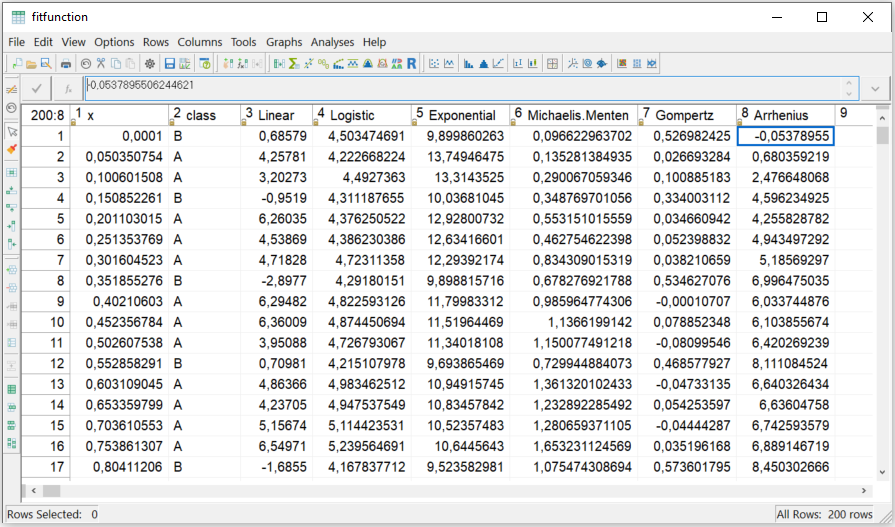
In this example, we start with the Cornerstone sample data set ‘fitfunction’. The data contains 200 simulated observations with random noise which can be fitted to the preselectable functions.

Fit Preselectable Function: Sample Data

We open the corresponding dataset in ‘Cornerstone’ and choose the menu ‘Analyses’ -> ‘CornerstoneR’ -> ‘Fit Function’ as shown in the following screenshot.

Fit Preselectable Function: Menu

In the appearing dialog, select variable ‘x’ to predictors. We choose ‘Logistic’ as the response variable at first. We want a fit for each group in the variable ‘class’ and select it as group by.

Fit Preselectable Function: Variable Selection

‘OK’ confirms your selection and the following window appears.

Fit Preselectable Function: R Script

Before we start the script, it is necessary to select the function we want to fit. To do this we open the menu ‘R Script’ -> ‘Script Variables’.

Fit Preselectable Function: R Script Variables Menu

In the appearing dialog we select the logistic function ‘Logistic’ instead of the default ‘User Defined’.

Fit Preselectable Function: R Script Variables

A selected function other than ‘User Defined’ gets its settings like predictor and response from the variable selection at the start. Additional settings like starting values use integrated calculations. Limits and Weights are topics in the ‘Special Situations’ chapter. ‘Maximum Iterations’ and ‘Maximum Error in SS’ are stop criteria and can be adjusted if needed.

Now close this dialog via ‘OK’ and click the execute button (green arrow) or choose the menu ‘R Script’ -> ‘Execute’ and all calculations are done via ‘R’. Calculations are done if the text at the lower left status bar contains ‘Last execute error state: OK’. Our result is available via the menus ‘Summaries’ as shown in the following screenshot.

Fit Preselectable Function: Result Menu

The menu ‘Convergence Information’ gives some information regarding the algorithm, e.g. if the algorithm converged (‘Converged’ is 1 if it did converge, and 0 otherwise), or how many iterations it took.

The menu ‘Coefficient Table’ gives the estimated coefficients of the function per group, together with their standard errors, pseudo R-squared and RMSE (Root Mean Square Error).

Fit Preselectable Function: Coefficients

The menu ‘Variance-Covariance Matrix of Coefficients’ shows the variance-covariance matrix of the coefficients for each group.

The menu ‘Fit Estimate’ opens a dataset with the group (‘class’), the original response (‘Logistic’), the fitted value (‘Fitted’), and the corresponding residuals (‘Residuals’). To visualize the function fit we can open the menu ‘Graph’ -> ‘x vs. Actual Fitted Values’ from the executed R script window. A scatter plot with ‘x’ as predictor, ‘Fitted’ as response, and ‘class’ as grouping variable appears.

Fit Preselectable Function: Fitted Data

Besides logistic, the same outputs can be computed using the other responses from the data and their related preselected functions. The predictor (‘x’) and the group by variable (‘class’) stay the same. The following screenshot shows the graph ‘x vs. Actual Fitted Values’…

…for the ‘Linear’ function,

Fit Preselectable Function: Linear

…for the ‘Exponential’ function,

Fit Preselectable Function: Exponential

…for the ‘Michaelis Menten’ function,

Fit Preselectable Function: Michaelis Menten

…for the ‘Gompertz’ function,

Fit Preselectable Function: Gompertz

… and for the ‘Arrhenius’ function.

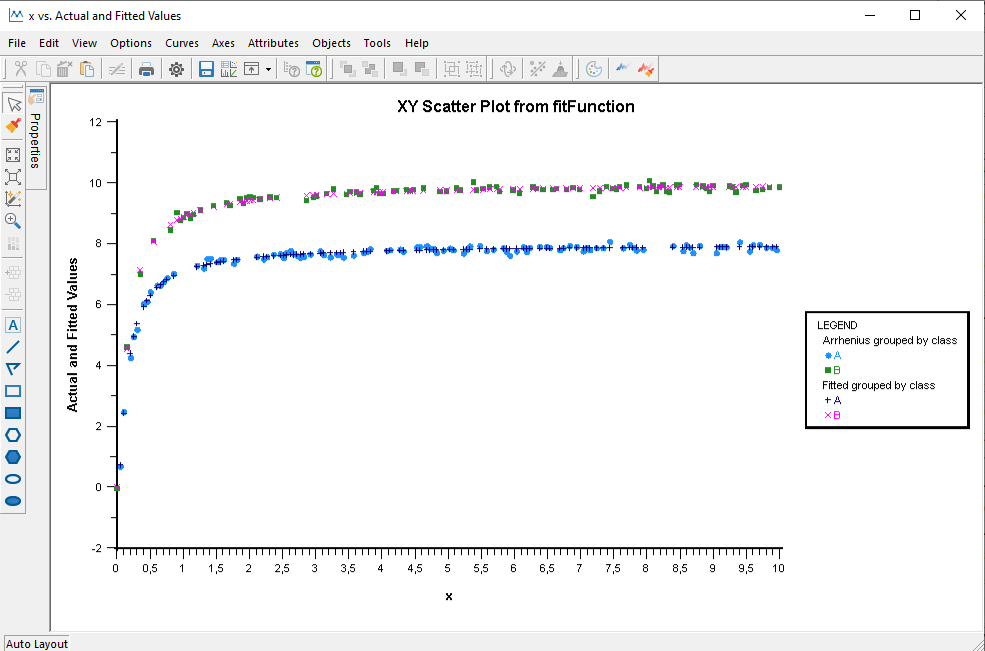
Fit Preselectable Function: Arrhenius

Fit User Defined Function

For this example we open the ‘Dissolution’ sample dataset in ‘Cornerstone’ from the ‘Regression’ subdirectory. This dataset is in wide format and we converted to long format using reshape grouped data to long. As a result we get a dataset like in the following screenshot. I renamed the columns ‘variable1’ and ‘variable2’ to ‘group1’ and ‘group2’ for a better identification.

Fit User Defined Function: Dissolution Data

From this dataset in ‘Cornerstone’ we start the to fit a function like in the first example via the menu ‘Analyses’ -> ‘CornerstoneR’ -> ‘Fit Function’. In the appearing dialog we select ‘Testtime’ as predictor, ‘value’ as response, and ‘group1’ and ‘group2’ as grouping variables like in the following screenshot.

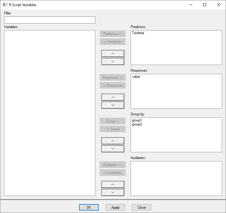
Fit User Defined Function: Variable Selection

After ‘OK’ the known ‘R Script’ dialog appears. Here we select the menu ‘R Script’ -> ‘Script Variables’ and use now the default setting ‘User Defined’ to fit a Weibull model to the Dissolution data.

Fit User Defined Function: Script Variables

The influence and target formula together form an equation of the form f(y)=g(x). In our case we set the prediction formula (right-hand side g(x)) to the formula of the Weibull model as shown in the screenshot. The response formula (left-hand side f(y)) is solely our response. For both text boxes we can use the button ‘<<’ and the drop-down box arranged on the left to add variables in a simple way. We can also add a function to the response formula like ‘log(value)’ if it improves the fit. As last step we set start values for each variable.

Now we close this dialog via ‘OK’ and execute the script (green arrow) by the menu ‘R Script’ -> ‘Execute’. One result is the dataset with all coefficients for the 24 groups as shown in the following screenshot.

Fit User Defined Function: Coefficient Table

From this dataset it is possible, for example, to create a multi-variable chart of the first coefficient, as shown in the following graph.

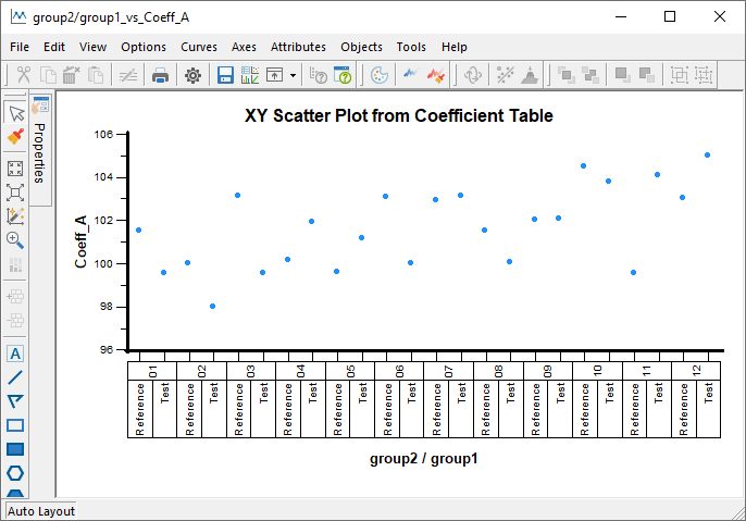
Fit User Defined Function: Multi-Vari Chart Coefficient ‘A’

Special Situations

This chapter briefly discusses special situations which can be handled via ‘fitFunction’.

Limits: Flattened Sinusoidal Oscillation

Assume a situation where your data looks like the curve in the following graph.

Fit Function: Flattened Sinusoidal Oscillation

Obviously the data is based on a sinusoidal oscillation which was censored, e.g., by a measuring instrument. The poor fit of a sinusoidal function is shown in the next graph.

Fit Function: Fitted Sinusoidal Oscillation

Limits reflect this behavior and can be handled like an additional coefficient. The following screenshot shows the use of a coefficient ‘c’ for the ‘min’ and ‘max’ limit.

Fit Function: Script Variables

The resulting fit is shown in the final graph.

Fit Function: Fitted Sinusoidal Oscillation with Limits

Weights: Small Example

Fitting a linear function (green) to data in a hyperbolic form (blue) results in the following graph.

Fit Function: Fit Linear Function on Hyperbolic Data

Generalizing the nonlinear least square algorithm to a weighted fit is done when you select a ‘Weight’ variable in the ‘Script Variables’ dialog as shown in the following screenshot.

Fit Function: Script Variables

The underlying variable contains a high weighting of data in the margin and a low weighting of data in the middle. This results in the following graph.

Fit Function: Weighted Linear Fit on Hyperbolic Data

The line is shifted accordingly by the weighting in the margin.